
The paper “Attention is All You Need” introduced the revolutionary Transformer model architecture. It was designed to overcome the limitations of the previously dominant architecture, the Recurrent Neural Network (RNN). Let’s explore the evolution, challenges with RNNs, and how Transformers address these issues.
RNN: The Predecessor to Transformers
RNNs were the go-to architecture for sequential data processing before Transformers came into existence.
Structure of RNN

An RNN consists of:
- An input layer, represented by X
- An output layer, represented by Y
- A hidden state initialized to zero at the start
The hidden states are passed from one neuron to the next as new inputs are fed, allowing the model to maintain context across sequences.
Challenges with RNNs
-
Slow Computation with Long Sequences:
As sequences grow, the process iterates repeatedly, making computation slower due to sequential dependencies. -
Vanishing or Exploding Gradients:
During training, the gradient values are multiplied across timesteps. If values are <1, they shrink (vanishing gradient); if >1, they grow exponentially (exploding gradient). Both hinder performance. For instance, multiplying 0.5 and 0.5 results in 0.25 - values diminish over time, leading to loss of learning signal. -
Difficulty Accessing Long-Term Dependencies:
Over long sequences, early inputs lose their influence due to repeated multiplications in the hidden states. This means information from earlier parts of the sequence is often “forgotten.”
The Transformer Architecture
The Transformer architecture introduces a novel approach by eliminating sequential dependencies, enabling faster and more efficient processing. It is divided into two main components:
- Encoder
- Decoder

Encoder
The encoder processes the input sequence and generates a contextual representation of it. It consists of several components:
-
Input Embedding:
The input text is tokenized, breaking it into smaller units like words or sub-words. For example:- Sentence: “Hello my name is Sourish”
- Tokenized: [“Hello”, “my”, “name”, “is”, “Sourish”] Each token is mapped to an Input ID (a numerical representation), e.g., “Hello” → 4535. These Input IDs are further embedded into a vector of size 512 (as defined in the paper: d_model = 512).
-
Positional Encoding:
The embeddings alone are insufficient as they do not capture the order of words. Positional Encoding adds a second vector of the same size (512) to encode information about the position of each word in the sentence. It ensures:- Words close to each other are treated as “close.”
- Words farther apart are treated as “distant.” The encoding is reusable across training and inference.
-
Multi-Head Attention:
Understanding Self-Attention: Self-attention helps the model relate words to one another. For example, in the sentence “Hello my name is Anmol,” the model identifies that “my” is more closely related to “Hello” than to “Anmol.” Mathematically, self-attention involves matrices Q (Query), K (Key), and V (Value). These matrices are derived from the input sentence. Each word creates its own Q, K, and V vectors by multiplying the input embedding with learned weight matrices. Self-attention calculates the importance of one word relative to the others by applying the following formula: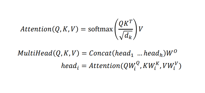
Multi-Head Attention:
Multi-head attention enhances the self-attention mechanism by splitting the Q, K, and V matrices into multiple smaller matrices (heads). Each head processes a portion of the data independently, focusing on different relationships within the sequence. Steps in Multi-Head Attention:- The input sequence, after positional encoding, is used to calculate Q, K, and V matrices.
- These matrices are split into smaller matrices for multiple heads.
- Each head independently computes attention scores using the self-attention formula.
- The outputs from all heads are concatenated and passed through a linear transformation to combine their insights.
This mechanism enables the model to analyze words in different contexts (e.g., a word being a noun, verb, or adjective).
-
Add & Norm:
After multi-head attention, a residual connection adds the input back to the output. Layer normalization is applied to stabilize learning by normalizing the values. Two parameters, γ (multiplicative) and β (additive), introduce necessary fluctuations in the data for better learning.
Decoder
The decoder generates the output sequence based on the encoder’s representations. It shares similar components with the encoder, with some differences:
-
Masked Multi-Head Attention:
To ensure causality, the decoder is masked so it cannot “see” future words in the output sequence during training. Future positions are replaced with -∞ in the attention matrix. -
Cross-Attention:
The decoder’s multi-head attention receives Keys (K) and Values (V) from the encoder, while Query (Q) comes from the decoder’s masked attention. This enables it to align with the encoder’s context.
Key Takeaways
The Transformer model eliminates the sequential dependency of RNNs, allowing parallelization and efficient processing of long sequences. Its components - including multi-head attention, positional encoding, and normalization - work together to revolutionize natural language processing tasks. From text generation to translation, the Transformer’s impact has been profound, making it the backbone of modern architectures like BERT and GPT.
This blog is based on the seminal paper “Attention is All You Need” by Vaswani et al. and insights from Umar Jamil’s explanatory video. Big thanks to the researchers for introducing Transformers and to Umar Jamil for breaking it down so well! 🚀